Autonomous Vehicle Motion Planner

Overview

The goal of this project is to build a motion planning stack for a self-driving car from scratch in C++. The car plans a global route with A*, generates smooth local trajectories in the Frenet frame, scores them, avoids obstacles, and drives itself to the goal. Everything runs in a 2D OpenCV simulation.

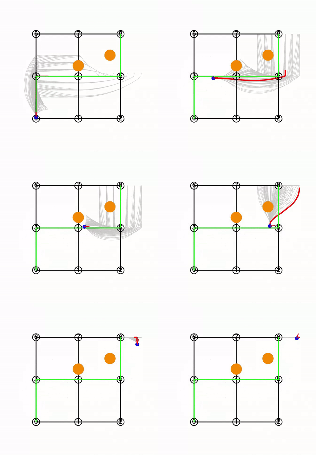
The planner driving the car around obstacles to the goal

The car follows the A* route, swerves around obstacles, and stops near the goal.

Blue = the car, green = the A* route, orange = obstacles, gray fan = candidate trajectories, bold red = the chosen collision-free trajectory.

Every layer was written and unit tested by hand without any planning libraries.

Planning Loop

The stack is split into three planning layers: global, local, and behavioral. They run in a loop on every frame.

Global route: A* searches a road graph for a path from start to goal.
Reference line: the jagged A* path becomes a smooth centerline with arc length and heading at every point.
Candidate generation: trajectories are sampled in the Frenet frame by sweeping lateral offset, time horizon, and target speed.
Scoring: every candidate gets a cost from jerk, lane center deviation, speed error, and obstacle proximity. The cheapest collision free one wins.
Behavior: a feasibility based state machine. CRUISE when a safe path exists, STOP when the road is blocked or the goal is reached.
Control: pure pursuit steering and proportional speed control execute the chosen trajectory on a kinematic bicycle model.

The planner then replans from the car’s new state.

The code is divided into several layers:

Layer	Responsibility	Code
Vehicle	Kinematic bicycle model	`vehicle/kinematic_model.*`
Global	Road graph and A* search	`planning/road_graph.`, `astar.`
Local	Frenet transforms, polynomials, cost	`planning/frenet.`, `_polynomial.*`
Behavioral	Feasibility based state machine	`planning/behavior.hpp`
Simulation	Render loop, controller, obstacles	`src/main.cpp`

Global Route

The road network is a graph of nodes (intersections) and bidirectional edges (road segments). A* searches it once at startup and uses straight line distance to the goal as the heuristic:

$$ f(n) = g(n) + h(n) $$

where:

$ f(n) $ : estimated total cost of a route passing through node $ n $
$ g(n) $ : cost already accumulated to reach $ n $
$ h(n) $ : Euclidean distance from $ n $ to the goal

The heuristic never overestimates the remaining cost, so A* returns the shortest route. The result is a list of waypoints. It describes which way to go, but it is too jagged for a car to drive.

The Frenet Frame

The local planner works in road relative coordinates $ (s, d) $ instead of world coordinates $ (x, y) $:

$ s $ : how far along the road the car is (arc length)
$ d $ : how far to the side of the centerline the car is (signed lateral offset)

The reference line is the smoothed A* route. A position is described by how far along it the car is ($ s $, green) and how far to the side it sits ($ d $, dashed), where $ \theta $ is the road heading at that point.

This turns a 2D curvy road problem into two 1D problems: make progress along the road, and pick a lane offset. A swerve becomes a single choice of $ d $ over time.

The A* waypoints are first converted into a reference line, a sequence of anchor points that each store a world position, the path tangent $ \theta $, and the cumulative arc length $ s $.

To convert a world point into Frenet coordinates, the planner finds the nearest reference point and projects the offset vector onto the road frame:

$$ s = s_{i} + \Delta \cdot \begin{bmatrix} \cos\theta \\ \sin\theta \end{bmatrix}, \qquad d = \Delta \cdot \begin{bmatrix} -\sin\theta \\ \cos\theta \end{bmatrix} $$

where:

$ i $ : index of the reference point nearest the query point
$ \Delta = (x - x_i,\ y - y_i) $ : vector from that reference point to the query point
$ s_i $ : arc length stored at that reference point
$ \theta $ : road heading at that reference point

The along track projection extends $ s $ past the anchor. The cross track projection gives the signed lateral offset, with $ +d $ to the left of the direction of travel.

The inverse transform interpolates a base point at arc length $ s $ between the two bracketing reference points, then steps $ d $ meters perpendicular to the interpolated heading:

$$ p_\mathrm{world} = p_\mathrm{ref}(s) + d \begin{bmatrix} -\sin\theta(s) \\ \cos\theta(s) \end{bmatrix} $$

where:

$ p_\mathrm{world} $ : the resulting world position
$ p_\mathrm{ref}(s) $ : point on the reference line at arc length $ s $, interpolated between the two bracketing anchors
$ \theta(s) $ : road heading at that same point

Trajectories often extend past the end of the reference line, so $ s $ is clamped to the range of the line before interpolating. Without the clamp there is no bracketing pair, the interpolation divides by zero, and the resulting NaN sends the car off the canvas.

Generating Candidate Trajectories

With the road flattened into $ (s, d) $, a trajectory is two independent functions of time. Both are minimum jerk so the motion stays smooth instead of twitchy.

Lateral Motion
A quintic polynomial is used because the lateral maneuver is fully constrained. The car starts at some offset and must arrive at a target offset with no lateral velocity or acceleration:

$$ d(t) = a_0 + a_1 t + a_2 t^2 + a_3 t^3 + a_4 t^4 + a_5 t^5 $$

where:

$ t $ : time since the start of the maneuver
$ T $ : the time horizon of the maneuver, meaning how long it lasts
$ a_0 $ to $ a_5 $ : coefficients solved from the boundary conditions

Six boundary conditions (position, velocity, and acceleration at $ t = 0 $ and $ t = T $) give six coefficients. The first three come directly from the start state. The remaining three are solved as a 3x3 linear system with Eigen.

Longitudinal Motion
A quartic polynomial is used because the car only needs to reach a cruising speed. Where it ends up along the road is left free:

$$ s(t) = a_0 + a_1 t + a_2 t^2 + a_3 t^3 + a_4 t^4 $$

Here $ a_0 $ to $ a_4 $ are the five coefficients of the longitudinal polynomial, and $ t $ and $ T $ mean the same as above. Dropping the end position constraint removes one equation, so the longitudinal polynomial is one degree lower than the lateral one.

The generator sweeps three axes to build the fan of candidates:

Lateral offset $ d $: ±3.0 m from the centerline, 7 samples
Time horizon $ T $: 2.0 to 5.0 s, 4 samples
Target speed: 5.0 ± 1.0 m/s, 3 samples

That gives 84 candidates per frame. Each one is sampled every 0.1 s and converted back to world coordinates for drawing and collision checking. This is the gray fan in the visualization.

Top: the fan produced from a single start state, bounded by the ±3 m road width. Bottom: the lateral curves must arrive at a chosen offset (six constraints, quintic), while the longitudinal curves only have to reach a speed and end up wherever they end up (five constraints, quartic).

Scoring

Every candidate gets a scalar cost and the cheapest collision free one wins:

$$ \begin{aligned} J = \ & w_j \sum_k \Big[ \big( \dddot{s}_k \big)^2 + \big( \dddot{d}_k \big)^2 \Big] \\ & + w_d\, d(T)^2 \\ & + w_v \big( \dot{s}(T) - v_\mathrm{target} \big)^2 \\ & + w_o \sum_k \sum_i \frac{1}{\max(\rho_{ki},\ \epsilon)} \end{aligned} $$

where:

$ J $ : total cost of one candidate, lower is better
$ k $ : index of a point along the trajectory, sampled every 0.1 s
$ i $ : index of an obstacle
$ T $ : the time horizon of the trajectory, so $ d(T) $ and $ \dot{s}(T) $ are values at the end of the maneuver
$ \dddot{s}_k,\ \dddot{d}_k $ : jerk along the road and across the road at point $ k $
$ v_\mathrm{target} $ : desired cruising speed (5 m/s)
$ \rho_{ki} $ : distance from point $ k $ to the edge of obstacle $ i $, which is the center distance minus the obstacle radius
$ \epsilon $ : a floor of 0.1 m so $ 1/\rho $ stays finite at the edge
$ w_j, w_d, w_v, w_o $ : the four weights, set to 1, 1, 1, and 5

Dots are time derivatives. One dot is speed, two dots is acceleration, and three dots is jerk, which is how abruptly the acceleration changes.

Each term encodes one preference:

Jerk: penalizes jolts on both axes, so comfortable trajectories win
Off center: pulls the car back to the lane center once it no longer needs to be elsewhere
Speed error: keeps the car near the target cruising speed
Obstacle proximity: inverse distance to each obstacle, so getting close is expensive even when it is not a collision

Squaring is used in the first three terms so that large errors count more than small ones and the sign does not matter. A drift of one meter left is penalized the same as one meter right.

The proximity term is what makes the avoidance look natural. A pure collision check is binary, so the car has no reason to move until a candidate actually hits an obstacle, which produces a late and sharp swerve. Inverse distance makes nearly hitting something expensive too, so the car starts drifting wide early. I set $ w_o $ to 5 times the other weights to prioritize early avoidance.

Collision checking inflates every obstacle by the radius of the car so each trajectory can be tested as a series of points. The extra margin also absorbs the tracking error of the pure pursuit controller.

Behavioral State Machine

The driving mode is a two state machine. How the state is decided mattered more than the states themselves.

CRUISE: a collision-free trajectory exists and the goal is not reached
STOP:   no collision-free trajectory, or the goal is reached

My first version decided the state by distance. A third SLOW state engaged when an obstacle came within a threshold, and STOP engaged when it came closer. This deadlocked immediately. Slowing down near an obstacle keeps the obstacle in range, which keeps the car slow, so a car that spawned near an obstacle froze at the start line and never moved.

The fix was to decide the state by feasibility. The Frenet planner already swerves around anything avoidable, so a nearby obstacle is not a reason to slow down. STOP means there is no way through, which happens when all 84 candidates collide. The SLOW state was removed.

Hollow dots are the skipped points and filled green dots are checked. The car cannot un-occupy where it already is, so judging those first points rejects every candidate at once.

A second deadlock came from the collision check itself. If the car drifted inside the inflated zone of an obstacle, every candidate started inside that zone and was flagged as a collision, so the car froze with nothing to follow. The collision check now skips the first few points of each trajectory, since only where a trajectory is going should count. A path that exits the zone stays valid and the car can drive back out.

Control

The chosen trajectory is executed on a kinematic bicycle model. It enforces non-holonomic motion, so the car cannot slide sideways and has a minimum turning radius the planner has to respect:

$$ \dot{x} = v\cos\theta, \qquad \dot{y} = v\sin\theta, \qquad \dot{\theta} = \frac{v}{L}\tan\delta $$

where:

$ v $ : the car’s speed
$ L $ : the wheelbase
$ \delta $ : the steering angle
$ \theta $ : the heading of the car in the world frame, not the road heading from the Frenet section
$ \dot{x},\ \dot{y} $ : how fast the car moves along each world axis
$ \dot{\theta} $ : how fast the car turns

Steering
Pure pursuit aims at a point 12 samples ahead on the freshly planned trajectory and steers by the heading error to that point, wrapped to $ [-\pi, \pi] $ so the car turns the short way. The trajectory is replanned every frame, so there is no need to track progress along the old plan.

The steering command is the angle between where the car is pointing and where the lookahead point sits.

Speed
A proportional controller sets the commanded acceleration $ a = K_p (v_\mathrm{desired} - v) $, where $ K_p $ is the gain. This is what makes the state machine reach the wheels. CRUISE targets the cruising speed and STOP targets zero.

Testing

Unit tests are written with Catch2 and cover the layers where a math error would be hard to spot from the visualization alone:

Road graph and A*: connectivity, shortest route correctness, and the case with no path.
Frenet transforms: arc length and heading along the reference line, signed lateral offset, and world to Frenet to world round trips.
Quintic and quartic polynomials: boundary conditions at $ t = 0 $ and $ t = T $, and matching derivatives.
Cost and collision: each penalty term responds in the right direction, and collision detection respects the inflated radius.

Tools

C++23
CMake
Eigen (solving for the polynomial coefficients)
OpenCV (2D visualization and render loop)
Catch2 v3 (unit tests)